
The article contains an overview of AI and machine learning applied in Chemistry along with libraries like RDKit.

Introduction
Machine learning models are poised to make a transformative impact on chemical sciences by dramatically accelerating computational algorithms and amplifying insights available from computational chemistry methods. However, achieving this requires a confluence and coaction of expertise in computer science and physical sciences.
One of the chief goals of chemistry is to understand the matter, its properties, and the transformations it can undergo. Chemistry is what we turn to when we are looking for a new superconductor, a vaccine, or any other material with the properties we desire.
Traditionally, we think of chemistry being done in a lab with test tubes, flasks, and gas burners. But it has also benefited from developments in computing and quantum mechanics, both of which rose to prominence in the early-mid 20th century. Early applications included using computers to help solve physics-based calculations; by blending theoretical chemistry with computer programming, we were able to simulate (albeit far from perfect) chemical systems. Eventually, this vein of work grew into a subfield now called computational chemistry. While computational chemistry has earned more and more glory over the past few decades, its importance has been largely overpowered by that of lab experiments - the cornerstone of chemical discovery.
However, with current improvements in AI, data-centric techniques, and ever-growing amounts of data, we might be witnessing a transition where computational techniques are used not just to aid lab experiments but to coach them.

AI Applications in Chemistry
While applications of Artificial Intelligence in the field of technology are immense, applications of artificial intelligence in chemical science are no less. Let us now have a look at some of the applications of Artificial Intelligence in the field of chemistry.
Detection of Molecular Properties
The first and foremost application of AI in chemistry is the detection of molecular properties. Scientists have been performing the process of detecting the chemical properties of molecules manually as identifying the properties of a molecule is a lengthy process.

Molecular property prediction. Credits
However, AI has facilitated this procedure and has enabled scientists to detect molecular properties. This has not only eased down the process of manual detection but has also made it more efficient for chemical procedures.
Moreover, detecting molecular properties has also enabled scientists to evaluate the potential of a hypothetical molecule. Artificial Intelligence algorithms have helped the field of chemistry to do as historical data empowers computers to analyze current data.
Designing Molecules
While the detection of molecular properties is extremely helpful in the field of chemistry, another use of artificial intelligence in molecular design has triggered revolutionary discoveries in the field.

Designing Molecules. Credits
Designing molecules has enabled scientists to gather historical data and synthesize chemical bonds for designing molecules. By incorporating AI algorithms, scholars have stepped ahead in discovering molecules that certainly help them to bring about revolutionary discoveries in ai chemical synthesis.
Furthermore, designing molecules leads to other useful applications too that have helped the field of chemistry to advance substantially.
Discovering Drugs
One of the topmost applications of Artificial Intelligence in Chemistry is the process of drug discovery. A revolutionary step in the realm of healthcare and science, the application of discovering drugs has proved to be highly useful.

Discovering Drugs. Credits
As new diseases are emerging on the surface, scientists are working hard toward the discovery of drugs in order to design new molecules and formulate effective medicines for curing fatal diseases.
Retrosynthesis Reaction
Retrosynthesis reaction is a process wherein molecules are broken down in order to determine their building blocks. As the term suggests itself, the process of synthesis (to produce something) is carried backward so as to discover a molecule's building blocks.

Retrosynthesis Reaction. Credits
Unlike contemporary times when scientists take the help of AI to conduct retrosynthesis reactions, scientists in the previous era used to conduct this process manually.
Tiresome and troublesome, this process was an extensive experience as it demanded a lot of time and resources. However, with the coming of Artificial Intelligence, this process can be conducted with the help of computers that have made it more accurate and efficient at the same time.
Predictive Analysis
Lastly, the application of ai in chemistry has helped scientists to gain predictive analysis. This is because with the help of historical data and by interpreting current data, computers generate advanced ai algorithms and patterns that represent predictive analysis for the future.
While such a prediction cannot be guaranteed, it still is highly accurate and efficient in terms of possibility and probability. With the help of Machine Learning or deep learning algorithms, computers are fed with data over time that improves their interpretation skills and empowers them to work along the lines of human intelligence.
Indeed, this application is highly crucial as it highlights the probable consequences or impact of certain chemical bonds, molecules, or even drugs that can guide the further steps in a positive direction.
Representation of chemical data
You might understand that in real-world chemistry we can find many examples of the things that are seeking to have a good data scientist look at. I'll tell the simplest ever example: two main general tasks that many chemistry researchers face almost every day are predicting the physical, chemical, biochemical (or some other desirable) properties of a molecule (or a substance when we talk about physical properties) by its general descriptors - chemical formula and 3D structure - and predicting chemical formula and 3D structure for an unknown yet molecule or substance with desirable properties respectively. They are called QSPR (quantitative structure-property relationship) and QSAR (quantitative structure-activity relationship) problems.
Let's consider a case where we want to implement some machine learning in chemistry research. The first issue we're going to face is how to represent the data in a way that keeps much information. When it comes to chemical formulas, in chemoinformatics there're several general ways of representation.
SMILES (Simplified Molecular Input Line Entry System)
This is the simplest way to reflect a molecule. The idea behind is to use simple line notations for chemical formulas that are based on some rules. Atoms of chemical elements are represented by chemical symbols in capital letters, hydrogen is usually ignored. Single bonds are not displayed; for double, triple, and quadruple bonds we shall use '=', '#', '$' respectively. Atoms that are bonded must stand nearby. Ring structures are written by breaking each ring at an arbitrary point (although some choices will lead to a more legible SMILES than others) to make a 'straight non-ring structure (as if it wasn't a ring) and adding numerical ring closure labels to show connectivity between non-adjacent atoms. Aromaticity is commonly illustrated by writing the constituent B, C, N, O, P, and S atoms in lower-case forms b, c, n, o, p and s, respectively. To represent side chains of atomic groups branches are used.
A simple example:

The fact that usually, you can find SMILES representation of a molecule in any database of chemical information makes the thing simple. But also you can write it by yourself if needed, which is definitely a huge advantage.

A complex example of SMILES representation of a molecule. Credits
Pros:
Easy to find or to write by yourself.
Illustrates some main chemical concepts such as atomic map, and bond structure, which can represent stereochemical properties (isomerism).
Can be further processed as string data, if needed.
Cons:
Doesn't give information on the spatial structure of the molecule (2D, but mostly 3D).
Different formulas may be written for the same molecule.
MDL Molfile
It's a file format that keeps the information about the atoms, bonds, connectivity, and coordinates of a molecule.
Typical MOL consists of some header information, the Connection Table containing atom info, then bond connections and types, followed by sections for more complex information. MOL representations can either hold information about the 2D or 3D structure of the molecule. This format is so widely spread that most cheminformatics software systems are able to read it.
Here is a MOL file for benzoic acid, generated by ChemDraw, which provides options to save or copy sketches in this file format.:

MOL file for benzoic acid. Credits
For a deeper understanding and interpretation of MDL Molfile, you can refer to this excellent blog.
Pros:
Acceptable by most chemoinformatics software.
Represents space structure (2D or 3D)
Invariant for a particular molecule.
Cons:
Huge size.
Can't be performed by yourself.
Coulomb matrices and other quantum descriptors
The Coulomb matrix as well as some custom quantum approaches come from the idea that molecular properties can be calculated from the Schrödinger equation, which takes the Hamiltonian operator as its input. The Hamiltonian operator for an isolated molecule can be specified by the atom coordinates and nuclear charges. In fact, there're many custom ways to represent a molecule with the help of quantum chemistry. The only limitation is the presence of such data.
Coulomb matrix is calculated with the equation below.

The diagonal elements can be seen as the interaction of an atom with itself and are essentially a polynomial fit of the atomic energies to the nuclear charge 𝑍𝑖Zi. The off-diagonal elements represent the Coulomb repulsion between nuclei 𝑖i and 𝑗j.
Let’s have a look at the Coulomb matrix for methanol:


In the matrix above the first row corresponds to carbon (C) in methanol interacting with all the other atoms (columns 2-5) and itself (column 1). Likewise, the first column displays the same numbers, since the matrix is symmetric. Furthermore, the second row (column) corresponds to oxygen and the remaining rows (columns) correspond to hydrogen (H).
Pros:
Mathematically and chemically strict representations.
Cons:
Hard to compute.
Seeks relative data.
Custom set of descriptors
One can actually represent the information by creating suitable descriptors that are believed to be helpful - bond count, atom count, presence of particular groups of atoms, etc. Such descriptors may be extracted from SMILES strings, MOL representations, or performed manually.
Pros:
Extracting suitable information based on chemical logic.
Cons:
Hard to produce manually.
Needs some other representation for computer processing.
May not represent a molecule correctly.
Apply Machine Learning on SMILES and MOL data representations
RDKit is a collection of cheminformatics and machine learning tools written in C++ and Python. What is more important, it allows you to work with many representations of chemical data and has the power to extract almost each chemical descriptor from the data you have. Check the docs for a deeper understanding.
In this tutorial, we'll try to implement ML to a prediction task. RDkit is the one to help at the first step. Or you can check my Kaggle notebook for all the steps.
!conda install -y -c rdkit rdkit;
!pip install pandas==0.23.0
Next, install all the basic libraries:
%matplotlib inline
import numpy as np
import pandas as pd
import matplotlib.pyplot as plt
import warningswarnings.filterwarnings("ignore")
We'll work with the data on lipophilicity of small organic molecules.
Lipophilicity is a physical property of a substance that refers to an ability of a chemical compound to dissolve in lipids, oils and generally in non-polar solvents. That's a fundamental property that plays great part in biochemical and technological behaviour of a substance. It's usually evaluated by a distribution coefficent P - the ratio of concentrations of a particular compound in a mixture of two immiscible phases at equilibrium (in our case water and octanol). The greater P values refer to greater lipophilicity. Usually lipophilicity is presented as log10P like in our dataset.
A thing important to mention is that it takes much time to perform an experiment to measure the corresponding P value, because it must be an exact and reproducible procedure repeated at least 3-5 times and each time you have to wait till the system's equilibrium is reached.
Chemical insights: from theory P value must turn great when a molecule is large and doesn't have many polar atoms or atomic groups (such containing O, N, P, S, Br, Cl, F an etc.) in it.
Let's load the dataset:
df= pd.read_csv('../input/mlchem/logP_dataset.csv', names=['smiles', 'logP'])
df.head()
As you see the only information we have here is SMILES representation of molecular formulas. But RDkit is able to work with MOL representations. And it's actually nice to know RDkit still provides an opportunity to transform SMILES to MOL. Let's check what we can do.
#Importing Chem module
from rdkit import Chem

#Method transforms smiles strings to mol rdkit object
df['mol'] = df['smiles'].apply(lambda x:Chem.MolFromSmiles(x))

#Now let's see what we've got
print(type(df['mol'][0]))
<class 'rdkit.Chem.rdchem.Mol'>Notice that MOLs are represented as special rdkit.Chem items of a corresponding C++ class.
Visualization of molecules
RDkit provides visualization of MOLs with rdkit.Chem.Draw module. To visualize a set of molecules you should pass a set of corresponging MOLs:
from rdkit.Chem import Draw

mols = df['mol'][:20]

#MolsToGridImage allows to paint a number of molecules at a time

Draw.MolsToGridImage(mols, molsPerRow=5, useSVG=True, legends=list(df['smiles'][:20].values))

Numbers of atoms
Since size of a molecule can be approximated by a number of atoms in it, let's extract corresponding values from MOL. RDkit provides GetNumAtoms() and GetNumHeavyAtoms() methods for that task.
# AddHs function adds H atoms to a MOL (as Hs in SMILES are usualy ignored)
# GetNumAtoms() method returns a general nubmer of all atoms in a molecule
# GetNumHeavyAtoms() method returns a nubmer of all atoms in a molecule with molecular weight > 1

df['mol'] = df['mol'].apply(lambda x: Chem.AddHs(x))
df['num_of_atoms'] = df['mol'].apply(lambda x: x.GetNumAtoms())
df['num_of_heavy_atoms'] = df['mol'].apply(lambda x: x.GetNumHeavyAtoms())
Let's take look at how number of atoms is connected with target variable:
import seaborn as sns

sns.jointplot(df.num_of_atoms, df.logP)
plt.show()
No clear dependence is observed so we need some more features to be exctracted. The next obvious step is to count numbers of the most common atoms. RDkit supports subpattern search represented by GetSubstructMatches() method. It takes a MOL of a substructure pattern as an argument. So you can futher extract occurance of each pattern you'd like.
# First we need to settle the pattern.
c_patt = Chem.MolFromSmiles('C')

# Now let's implement GetSubstructMatches() method
print(df['mol'][0].GetSubstructMatches(c_patt))
((0,), (1,), (2,), (3,))The method returns a tuple of tuples of positions of corresponding patterns. To extract the number of matches we need to take the length of a corresponding tuple of tuples.
#We're going to settle the function that searches patterns and use it for a list of most common atoms only

def number_of_atoms(atom_list, df):
    for i in atom_list:
        df['num_of_{}_atoms'.format(i)] = df['mol'].apply(lambda x:     len(x.GetSubstructMatches(Chem.MolFromSmiles(i))))

number_of_atoms(['C','O', 'N', 'Cl'], df)sns.pairplot(df[['num_of_atoms','num_of_C_atoms','num_of_N_atoms', 'num_of_O_atoms', 'logP']], diag_kind='kde', kind='reg', markers='+')
plt.show()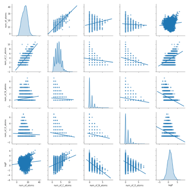
Looking at the bottom plots we notice some linear dependence of logP on numbers of particular atoms. We also see normal distribution of the target variable which values lie approximately from -5 to 5.
Let's build our first model. We'll count on ridge regression.
from sklearn.linear_model import RidgeCV
from sklearn.model_selection import train_test_split

#Leave only features columns
train_df = df.drop(columns=['smiles', 'mol', 'logP'])
y = df['logP'].values

print(train_df.columns)

#Perform a train-test split. We'll use 10% of the data to evaluate the model while training on 90%

X_train, X_test, y_train, y_test = train_test_split(train_df, y, test_size=.1, random_state=1)
Index(['num_of_atoms', 'num_of_heavy_atoms', 'num_of_C_atoms',
       'num_of_O_atoms', 'num_of_N_atoms', 'num_of_Cl_atoms'],
      dtype='object')
Train the model and evaluate results. As an evaluation metric we can choose MAE or MSE. Evaluation function plots a number of first predictions (by default - 300).
from sklearn.metrics import mean_absolute_error, mean_squared_error

def evaluation(model, X_test, y_test):

    prediction = model.predict(X_test)
    mae = mean_absolute_error(y_test, prediction)
    mse = mean_squared_error(y_test, prediction)

    plt.figure(figsize=(15, 10))
    plt.plot(prediction[:300], "red", label="prediction",     linewidth=1.0)
    plt.plot(y_test[:300], 'green', label="actual", linewidth=1.0)
    plt.legend()
    plt.ylabel('logP')
    plt.title("MAE {}, MSE {}".format(round(mae, 4), round(mse, 4)))
    plt.show()

    print('MAE score:', round(mae, 4))
    print('MSE score:', round(mse,4))
#Train the model
ridge = RidgeCV(cv=5)
ridge.fit(X_train, y_train)
#Evaluate results
evaluation(ridge, X_test, y_test)
MAE score: 0.5724
MSE score: 0.5398
Offtop: particular atoms, bonds and rings
Note that you can also extract some ring information or iterate through each molecule's atoms and bonds with RDkit. Methods GetRingInfo(), GetAtoms() and GetBonds() yield corresponding generators over rings and atoms in molecule.
Some toy examples:
atp = Chem.MolFromSmiles('C1=NC2=C(C(=N1)N)N=CN2[C@H]3[C@@H]([C@@H]([C@H](O3)COP(=O)(O)OP(=O)(O)OP(=O)(O)O)O)O')

# Getting number of rings with specified number of backbones
print('Number of rings with 1 backbone:', atp.GetRingInfo().NumAtomRings(1))
print('Number of rings with 2 backbones:', atp.GetRingInfo().NumAtomRings(2))
Number of rings with 1 backbone: 1
Number of rings with 2 backbones: 2
m = Chem.MolFromSmiles('C(=O)C(=N)CCl')

#Iterating through atoms to get atom symbols and explicit valencies for atom in m.GetAtoms():
    print('Atom:', atom.GetSymbol(), 'Valence:',  atom.GetExplicitValence())
Atom: C Valence: 3
Atom: O Valence: 2
Atom: C Valence: 4
Atom: N Valence: 2
Atom: C Valence: 2
Atom: Cl Valence: 1
Descriptors
rdkit.Chem.Descriptors provides a number of general molecular descriptors that can also be used to featurize a molecule. Most of the descriptors are straightforward to use from Python.
Using this package we can add some useful features to our model:
rdkit.Chem.Descriptors.TPSA() - the surface sum over all polar atoms or molecules also including their attached hydrogen atoms;
rdkit.Chem.Descriptors.ExactMolWt() - exact molecural weight;
rdkit.Chem.Descriptors.NumValenceElectrons() - number of valence electrons (may illustrate general electronic density)
rdkit.Chem.Descriptors.NumHeteroatoms() - general number of non-carbon atoms.
from rdkit.Chem import Descriptors

df['tpsa'] = df['mol'].apply(lambda x: Descriptors.TPSA(x))
df['mol_w'] = df['mol'].apply(lambda x: Descriptors.ExactMolWt(x))
df['num_valence_electrons'] = df['mol'].apply(lambda x: Descriptors.NumValenceElectrons(x))
df['num_heteroatoms'] = df['mol'].apply(lambda x: Descriptors.NumHeteroatoms(x))
Let's check the improvement of the model perfomance with new features.
train_df = df.drop(columns=['smiles', 'mol', 'logP'])
y = df['logP'].values
print(train_df.columns)

#Perform a train-test split. We'll use 10% of the data to evaluate the model while training on 90%
X_train, X_test, y_train, y_test = train_test_split(train_df, y, test_size=.1, random_state=1)
Index(['num_of_atoms', 'num_of_heavy_atoms', 'num_of_C_atoms',
'num_of_O_atoms', 'num_of_N_atoms', 'num_of_Cl_atoms', 'tpsa', 'mol_w',
'num_valence_electrons', 'num_heteroatoms'],
dtype='object')
#Train the model
ridge = RidgeCV(cv=5)
ridge.fit(X_train, y_train)

#Evaluate results and plot predictions
evaluation(ridge, X_test, y_test)
MAE score: 0.4629
MSE score: 0.3525
RDkit is a wonderful tool to work with chemical data, especially represented as SMILES strings or in MOL format. We've seen some basic general abilities of the package but some other powerful tools are yet to be found in the docs.
Classification of HIV virus
Now lets deal with a classification problem. We'll use a dataset from MoleculeNet database - a benchmark for computional chemistry. There's a number of datasets for classification, so I've picked the one that is not so large - HIV dataset. From description: "The HIV dataset was introduced by the Drug Therapeutics Program (DTP) AIDS Antiviral Screen, which tested the ability to inhibit HIV replication for over 40,000 compounds. Screening results were evaluated and placed into three categories: confirmed inactive (CI),confirmed active (CA) and confirmed moderately active (CM). We further combine the latter two labels, making it a classification task between inactive (CI) and active (CA and CM)".
In the dataset once again we can find SMILES representations and two target columns, but only 'HIV_active' is used as a benchmark. A benchmark for Logistic Regression for this task is ROC AUC = 0.782.
import warnings
warnings.filterwarnings("ignore")

#Read the data
hiv = pd.read_csv('../input/mlchem/HIV.csv')
hiv.head()
#Let's look at the target values count
sns.countplot(data = hiv, x='HIV_active', orient='v')
plt.ylabel('HIM active')
plt.xlabel('Count of values')
plt.show()
We notice great class disbalance. Now let's repeat the same approaches. At the first step - descriptors from RDkit.
#Transform SMILES to MOL
hiv['mol'] = hiv['smiles'].apply(lambda x: Chem.MolFromSmiles(x))

#Extract descriptors
hiv['tpsa'] = hiv['mol'].apply(lambda x: Descriptors.TPSA(x))
hiv['mol_w'] = hiv['mol'].apply(lambda x: Descriptors.ExactMolWt(x))
hiv['num_valence_electrons'] = hiv['mol'].apply(lambda x: Descriptors.NumValenceElectrons(x))
hiv['num_heteroatoms'] = hiv['mol'].apply(lambda x: Descriptors.NumHeteroatoms(x))
Train and evaluate the model.
y = hiv.HIV_active.values
X = hiv.drop(columns=['smiles', 'activity','HIV_active', 'mol'])

X_train, X_test, y_train, y_test = train_test_split(X, y, test_size=.20, random_state=1)
from sklearn.metrics import auc, roc_curve

def evaluation_class(model, X_test, y_test):
    prediction = model.predict_proba(X_test)
    preds = model.predict_proba(X_test)[:,1]
    fpr, tpr, threshold = roc_curve(y_test, preds)
    roc_auc = auc(fpr, tpr)

    plt.title('ROC Curve')
    plt.plot(fpr, tpr, 'g', label = 'AUC = %0.3f' % roc_auc)
    plt.legend(loc = 'lower right')
    plt.plot([0, 1], [0, 1],'r--')
    plt.xlim([0, 1])
    plt.ylim([0, 1])
    plt.ylabel('True Positive Rate')
    plt.xlabel('False Positive Rate')
    plt.show()

    print('ROC AUC score:', round(roc_auc, 4))
from sklearn.linear_model import LogisticRegression
from sklearn.preprocessing import StandardScaler
X_train = StandardScaler().fit_transform(X_train)
X_test = StandardScaler().fit_transform(X_test)
lr = LogisticRegression()
lr.fit(X_train, y_train)
evaluation_class(lr, X_test, y_test)
ROC AUC score: 0.6945
And finally let's add molecular embeddings with mol2vec.
#Constructing sentences
hiv['sentence'] = hiv.apply(lambda x: MolSentence(mol2alt_sentence(x['mol'], 1)), axis=1)

#Extracting embeddings to a numpy.array
#Note that we always should mark unseen='UNK' in sentence2vec() so that model is taught how to handle unknown substructures
hiv['mol2vec'] = [DfVec(x) for x in sentences2vec(hiv['sentence'], model, unseen='UNK')]
X_mol = np.array([x.vec for x in hiv['mol2vec']])
X_mol = pd.DataFrame(X_mol)

#Concatenating matrices of features
new_hiv = pd.concat((X, X_mol), axis=1)
X_train, X_test, y_train, y_test = train_test_split(new_hiv, y, test_size=.20, random_state=1)

X_train = StandardScaler().fit_transform(X_train)
X_test = StandardScaler().fit_transform(X_test)

lr = LogisticRegression()
lr.fit(X_train, y_train)

evaluation_class(lr, X_test, y_test

ROC AUC score: 0.7896 That's an absolutely outstanding result when comparing to best results on MoleculeNet. Even though we were unable to reproduce the split, still results show that we are very close to or even better than best results published on MoleculeNet. Incredible!
Conclusion
We've tried a number of approaches to handle chemical data and built rather good predictive models for physical and biological properties of chemical matter with wonderful RDkit = packages. I suppose further feature construction can bring an even better result, but still, it's shown that we are able to predict important general properties rather fast and easy, without constructing great neural networks or spending weeks on quantum calculations, which can actually be implemented in a lab if an approximated evaluation of the target is needed. Another important outcome is the fact that these approaches are suitable for both regression and classification tasks (in the classification task we dealt to beat a MoleculeNet benchmark).
References
Kaggle Datasets: LogP of Chemical Structures: https://www.kaggle.com/matthewmasters/chemical-structure-and-logp
Jaeger, S., Fulle, S., & Turk, S. (2018). Mol2vec: Unsupervised machine learning approach with chemical intuition. Journal of chemical information and modeling, 58(1), 27-35. URL = {http://dx.doi.org/10.1021/acs.jcim.7b00616}, eprint = {http://dx.doi.org/10.1021/acs.jcim.7b00616}
Comments