
Learn how to build a Language Translator using Encoder-Decoder architecture.

Introduction
We all are familiar with Google translator and have probably already used it. But have you ever wondered how come it translates almost any known language into the language of our choice?
So in this article, we are going to decode this mystery and learn how to build a language translator using Enoder-Decoder architecture. Before moving forward I would suggest you guys go through LSTM, and learn more about it, from here.
I have broken this article into two parts. The first part consists of a brief explanation of NMT and the Encoder-Decoder structure. Following this, the second part of the article provides a step by step approach to create a language translator yourself using Python.
So let's get started and understand the core concepts involved.
What are Machine Translation(MT) and Neural Machine Translation(NMT)?
Machine translation(MT) is a subfield of computational linguistics that is focused on the task of automatically converting source text in one language to text in another language.
In machine translation, the input already consists of a series of symbols in some language, and the computer program must convert this into a series of symbols in a different language.
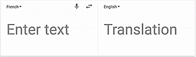
Google Translator
Neural machine translation (NMT) is a proposition to machine translation that uses an artificial neural network to predict the probability of a sequence of words, typically modeling whole sentences in a single integrated model.
With the power of Neural networks, Neural Machine Translation (NMT) has emerged as the most powerful algorithm to perform this task. This state-of-the-art algorithm is an application of deep learning in which massive datasets of translated sentences are used to train a model capable of translating between any two languages.
Understand the Sequence to Sequence (Seq2Seq) Architecture
As the name suggests, seq2seq takes as input a sequence of words(sentence or sentences) and generates an output sequence of words. It does so by the use of the recurrent neural network (RNN). The idea is to use 2 RNN that will work together with a special token and trying to predict the next state sequence from the previous sequence.

It mainly has two components i.e encoder and decoder, and hence sometimes it is called the Encoder-Decoder Network.
Encoder: It uses deep neural network layers and converts the input words to corresponding hidden vectors. Each vector represents the current word and the context of the word.
Decoder: It is similar to the encoder. It takes as input the hidden vector generated by the encoder, its own hidden states, and current word to produce the next hidden vector and finally predict the next word.
The ultimate goal of any NMT model is to take input a sentence in one language and return that sentence translated into a different language as output.
The figure below is a naive representation of a translation algorithm trained for translating from Chinese to English.
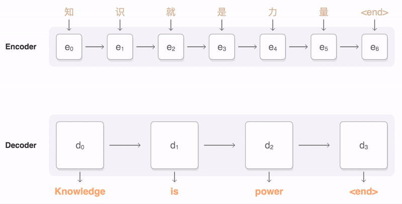
Encoder-Decoder in action. Credits
How Encoder-Decoder architecture work?
The first step is to somehow convert our textual data into a numeric form. To do this in machine translation, each word is transformed into a One Hot Encoding vector which can then be inputted into the model. A-One Hot Encoding vector is simply a vector with a 0 at every index except for a 1 at a single index corresponding to that particular word.

One Hot Encoding. Credits
These vectors are created by assigning an index to each unique word in the input language, and then repeat this process for the output language. In assigning a unique index to each unique word, we will be creating what is referred to as a Vocabulary for each language. Ideally, the Vocabulary for each language would simply contain every unique word in that language.

As you can see above, each word becomes a vector of length 9(which is the size of our vocabulary) and consists entirely of 0s except for a 1 at the index.
By creating a vocabulary for both the input and output languages, we can perform this technique on every sentence in each language to completely transform any corpus of translated sentences into a format suitable for the task of machine translation.
Let us now look at the magic behind this Encoder-Decoder algorithm. At the most basic level, the Encoder portion of the model takes a sentence in the input language and creates a thought vector from this sentence. This thought vector stores the meaning of the sentence and is subsequently passed to a Decoder which outputs the translation of the sentence in the output language.

In the case of the Encoder, each word in the input sentence is fed separately into the model in a number of consecutive time-steps. At each time-step, t, the model updates a hidden vector, h,using information from the word inputted to the model at that time-step. This hidden vector works to store information about the inputted sentence. In this way, since no words have yet been inputted to the Encoder at time-step t=0, the hidden state in the Encoder starts out as an empty vector at this time-step. The hidden state is represented with the blue box in the below figure, where the subscript t=0 indicates the time-step and the superscript E corresponds to the fact that it’s a hidden state of the Encoder (rather than a D for the Decoder).

At each time-step, this hidden vector takes in information from the inputted word at that time-step, while preserving the information it has already stored from previous time-steps. Thus, at the final time-step, the meaning of the whole input sentence is stored in the hidden vector. This hidden vector at the final time-step is the thought vector referred to above, which is then inputted into the Decoder.
Also, notice how the final hidden state of the Encoder becomes the thought vector and is relabeled with superscript D at t=0. This is because this final hidden vector of the Encoder becomes the initial hidden vector of the Decoder. In this way, we are passing the encoded meaning of the sentence to the Decoder to be translated to a sentence in the output language. However, unlike the Encoder, we need the Decoder to output a translated sentence of variable length. Thus, we are going to have our Decoder output a prediction word at each time-step until we have outputted a complete sentence.
In order to start this translation, we are going to input a <SOS> tag as the input at the first time-step in the Decoder. Just as in the Encoder, the Decoder will use the <SOS> input at time-step t=1 to update its hidden state. However, rather than just proceeding to the next time-step, the Decoder will use an additional weight matrix to create a probability over all of the words in the output vocabulary. In this way, the word with the highest probability in the output vocabulary will become the first word in the predicted output sentence.
The Decoder has to output prediction sentences of variable lengths, the Decoder will continue predicting words in this fashion until it predicts the next word in the sentence to be a <EOS> tag. Once this tag has been predicted, the decoding process is complete and we are left with a complete predicted translation of the input sentence.
Python Implementation of NMT using Keras
Now that we understood the encoder-decoder architecture, let's create a model that will translate English sentences into their French-language counterparts using Keras and python.
As a first step, we will import the required libraries and will configure values for different parameters that we will be using in the code. Let’s first import the required libraries:
#Import Libraries
import os,sys
from keras.models import Model
from keras.layers import Input, LSTM, GRU, Dense, Embedding
from keras.preprocessing.text import Tokenizer
from keras.preprocessing.sequence import pad_sequences
from keras.utils import to_categorical
import numpy as np
import pandas as pd
import pickle
import matplotlib.pyplot as plt

#Values for different parameters:
BATCH_SIZE=64
EPOCHS=20
LSTM_NODES=256
NUM_SENTENCES=20000
MAX_SENTENCE_LENGTH=50
MAX_NUM_WORDS=20000
EMBEDDING_SIZE=200
The Dataset
We need a dataset that contains English sentences and their French translations which can be freely downloaded from this link. Download the file fra-eng.zip and extract it. On each line, the text file contains an English sentence and its French translation, separated by a tab.
Let’s go ahead and split each line into input text and target text.
input_sentences= []
output_sentences= []
output_sentences_inputs= []
count=0
for line in open('./drive/My Drive/fra.txt', encoding="utf-8"):
    count+=1
    if count > NUM_SENTENCES:
        break
    if '\t' not in line:
        continue
    input_sentence = line.rstrip().split('\t')[0]
    output=line.rstrip().split('\t')[1]
    output_sentence=output+' <eos>'
    output_sentence_input='<sos>'+output

    input_sentences.append(input_sentence)
    output_sentences.append(output_sentence)
    output_sentences_inputs.append(output_sentence_input)

print("Number of sample input:", len(input_sentences))
print("Number of sample output:", len(output_sentences))
print("Number of sample output input:", len(output_sentences_inputs))
Output:
Number of sample input: 20000
Number of sample output: 20000
Number of sample output input: 20000In the script above we created three lists input_sentences[], output_sentences[], and output_sentences_inputs[]. Next, in the for loop the fra.txt file is read one line at a time. Each line is split into two substrings at the position where the tab occurs. The left substring (the English sentence) is inserted into the input_sentences[] list. The substring to the right of the tab is the corresponding translated French sentence.
Here, the <eos> token, which denotes the end-of-sentence is prefixed to the translated sentence. Similarly, the <sos> token, which denotes for "start of the sentence", is concatenated at the start of the translated sentence.
Let us also print a random sentence from the lists:
print("English sentence: ",input_sentences[180])
print("French translation: ",output_sentences[180])

Output:
English sentence:  Join us.
French translation:  Joignez-vous à nous. <eos>
Tokenization and Padding
The next step is tokenizing the original and translated sentences and applying padding to the sentences that are longer or shorter than a certain length, which in case of inputs will be the length of the longest input sentence. And for the output, this will be the length of the longest sentence in the output.
But before we do that, let’s visualize the length of the sentences. We will capture the lengths of all the sentences in two separate lists for English and French, respectively.
eng_len= []
fren_len= []# populate the lists with sentence lengths
for i in input_sentences:
    eng_len.append(len(i.split()))

for i in output_sentences:
    fren_len.append(len(i.split()))

length_df=pd.DataFrame({'english':eng_len, 'french':fren_len})

length_df.hist(bins=20)
plt.show()
The histogram above shows the maximum length of the French sentences is 12 and that of the English sentence is 6.
Next, vectorize our text data by using Keras’s Tokenizer() class. It will turn our sentences into sequences of integers. We can then pad those sequences with zeros to make all the sequences of the same length.
#tokenize the input sentences(input language) input_tokenizer=Tokenizer(num_words=MAX_NUM_WORDS)
input_tokenizer.fit_on_texts(input_sentences)
input_integer_seq=input_tokenizer.texts_to_sequences(input_sentences)
print(input_integer_seq)

word2idx_inputs = input_tokenizer.word_indexprint('Total unique words in the input: %s'%len(word2idx_inputs))

max_input_len = max(len(sen) for sen in input_integer_seq)

print("Length of longest sentence in input: %g"%max_input_len)
The word_index attributes of the Tokenizer class return a word-to-index dictionary where the keys represent words and the values represent corresponding integers. Finally, the above script prints the number of unique words in the dictionary and the length of the longest sentence in the input English language.
Output:
Total unique words in the input: 3501
Length of longest sentence in input: 6
Likewise, the output sentences can also be tokenized in the same way:
#tokenize the output sentences(Output language)
output_tokenizer = Tokenizer(num_words=MAX_NUM_WORDS, filters='')
output_tokenizer.fit_on_texts(output_sentences+output_sentences_inputs)
output_integer_seq = output_tokenizer.texts_to_sequences(output_sentences)
output_input_integer_seq = output_tokenizer.texts_to_sequences(output_sentences_inputs)
print(output_input_integer_seq)

word2idx_outputs = output_tokenizer.word_index
print('Total unique words in the output: %s' % len(word2idx_outputs))

num_words_output = len(word2idx_outputs) + 1
max_out_len = max(len(sen) for sen in output_integer_seq)
print("Length of longest sentence in the output: %g" % max_out_len)
Output:
Total unique words in the output: 9511
Length of longest sentence in the output: 12Now the lengths of the longest sentences in both the language can be verified from the histogram above. It can also be concluded that English sentences are normally shorter and contain a smaller number of words on average, compared to the translated French sentences.
Next, we need to pad the input. The reason behind padding the input and the output is that text sentences can be of varying length, however LSTM expects input instances with the same length. Therefore, we need to convert our sentences into fixed-length vectors. One way to do this is via padding.
#Padding the encoder input
encoder_input_sequences=pad_sequences(input_integer_seq, maxlen=max_input_len)
print("encoder_input_sequences.shape:", encoder_input_sequences.shape)

#Padding the decoder inputs
decoder_input_sequences=pad_sequences(output_input_integer_seq, maxlen=max_out_len, padding='post')
print("decoder_input_sequences.shape:", decoder_input_sequences.shape)

#Padding the decoder outputs
decoder_output_sequences=pad_sequences(output_integer_seq, maxlen=max_out_len, padding='post')
print("decoder_output_sequences.shape:", decoder_output_sequences.shape)
Output:
encoder_input_sequences.shape: (20000, 6)
decoder_input_sequences.shape: (20000, 12)
decoder_output_sequences.shape: (20000, 12)
Since there are 20,000 sentences in the input(English) and each input sentence is of length 6, the shape of the input is now (20000, 6). Similarly, there are 20,000 sentences in the output(French) and each output sentence is of length 12, the shape of the input is now (20000, 12) and the same goes for translated language.
You may recall that the original sentence at index 180 is join us. The tokenizer divided the sentence into two words join and us, converted them to integers, and then applied pre-padding by adding four zeros at the start of the corresponding integer sequence for the sentence at index 180 of the input list.
print("encoder_input_sequences[180]:", encoder_input_sequences[180])

Output:
encoder_input_sequences[180]: [  0   0   0   0 464  59]
To verify that the integer values for join and us are 464 and 59 respectively, you can pass the words to the word2index_inputs dictionary, as shown below:
print(word2idx_inputs["join"])
print(word2idx_inputs["us"])

Output:
464
59
It is further important to mention that in the case of the decoder, the post-padding is applied, which means that zeros are appended at the end of the sentence. In the encoder, zeros were padded at the beginning. The reason behind this approach is that encoder output is based on the words occurring at the end of the sentence, therefore the original words were kept at the end of the sentence, and zeros were padded at the beginning. On the other hand, in the case of the decoder, the processing starts from the beginning of a sentence, and therefore post-padding is performed on the decoder inputs and outputs.
Word Embeddings
We always have to convert our words into their corresponding numeric vector representations before feeding it to any deep learning model and we already converted our words into numeric. So what’s the difference between integer/numeric representation and word embeddings?
There are two main differences between single integer representation and word embeddings. With integer representation, a word is represented only with a single integer. With vector representation, a word is represented by a vector of 50, 100, 200, or whatever dimensions you like. Hence, word embeddings capture a lot more information about words. Secondly, the single-integer representation doesn’t capture the relationships between different words. On the contrary, word embeddings retain relationships between the words.
For English sentences, i.e. the inputs, we will use the GloVe word embeddings. For the translated French sentences in the output, we will use custom word embedding. You can download GloVe word embedding from here.
Let’s create word embeddings for the inputs first. To do so, we need to load the GloVe word vectors into memory. We will then create a dictionary where words are the keys and the corresponding vectors are values,
from numpy import array
from numpy import asarray
from numpy import zeros

embeddings_dictionary = dict()

glove_file = open(r'./drive/My Drive/glove.twitter.27B.200d.txt', encoding="utf8")

for line in glove_file:
    rec = line.split()
    word = rec[0]
    vector_dimensions = asarray(rec[1:], dtype='float32')
    embeddings_dictionary[word] = vector_dimensions

glove_file.close()
Recall that we have 3501 unique words in the input. We will create a matrix where the row number will represent the integer value for the word and the columns will correspond to the dimensions of the word. This matrix will contain the word embeddings for the words in our input sentences.
num_words = min(MAX_NUM_WORDS, len(word2idx_inputs) +1)

embedding_matrix = zeros((num_words, EMBEDDING_SIZE))
for word, index in word2idx_inputs.items():
    embedding_vector=embeddings_dictionary.get(word)
    if embedding_vector is not None:
        embedding_matrix[index] =embedding_vector
Creating the Model
The first step is to create an Embedding layer for our neural network.
The Embedding layer is defined as the first hidden layer of a network. It must specify 3 arguments:
input_dim: This is the size of the vocabulary in the text data. For example, if your data is integer encoded to values between 0–10, then the size of the vocabulary would be 11 words.
output_dim: This is the size of the vector space in which words will be embedded. It defines the size of the output vectors from this layer for each word. For example, it could be 32 or 100 or even larger. Test different values for your problem.
input_length: This is the length of input sequences, as you would define for any input layer of a Keras model. For example, if all of your input documents are comprised of 1000 words, this would be 1000.
embedding_layer = Embedding(num_words, EMBEDDING_SIZE, weights=[embedding_matrix], input_length=max_input_len)The next thing we need to do is to define our outputs, as we know that the output will be a sequence of words. Recall that the total number of unique words in the output is 9511. Therefore, each word in the output can be any of the 9511 words. The length of an output sentence is 12. And for each input sentence, we need a corresponding output sentence. Therefore, the final shape of the output will be:
(number of inputs, length of the output sentence, the number of words in the output)
#shape of the output
decoder_targets_one_hot = np.zeros((len(input_sentences), max_out_len, num_words_output),
dtype='float32'
)

decoder_targets_one_hot.shape

Shape:
(20000, 12, 9512)
To make predictions, the final layer of the model will be a dense layer, therefore we need the outputs in the form of one-hot encoded vectors since we will be using softmax activation function at the dense layer. To create such one-hot encoded output, the next step is to assign 1 to the column number that corresponds to the integer representation of the word.
for i, d in enumerate(decoder_output_sequences):
    for t, word in enumerate(d):
        decoder_targets_one_hot[i, t, word] = 1
The next step is to define the encoder and decoder network.
The input to the encoder will be the sentence in English and the output will be the hidden state and cell state of the LSTM.
encoder_inputs=Input(shape=(max_input_len,))
x=embedding_layer(encoder_inputs)
encoder=LSTM(LSTM_NODES, return_state=True)

encoder_outputs, h, c=encoder(x)
encoder_states= [h, c]
The next step is to define the decoder. The decoder will have two inputs: the hidden state and cell state from the encoder and the input sentence, which actually will be the output sentence with a token appended at the beginning.
decoder_inputs=Input(shape=(max_out_len,))
decoder_embedding=Embedding(num_words_output, LSTM_NODES)
decoder_inputs_x=decoder_embedding(decoder_inputs)

decoder_lstm=LSTM(LSTM_NODES, return_sequences=True, return_state=True)
decoder_outputs, _, _=decoder_lstm(decoder_inputs_x, initial_state=encoder_states)

#Finally, the output from the decoder LSTM is passed through a dense layer to predict decoder outputs.
decoder_dense=Dense(num_words_output, activation='softmax')
decoder_outputs=decoder_dense(decoder_outputs)
Training the Model
Let’s compile the model defining the optimizer and our cross-entropy loss.
#Compile
model=Model([encoder_inputs,decoder_inputs], decoder_outputs)

model.compile(optimizer='rmsprop',loss='categorical_crossentropy',metrics=['accuracy'])

model.summary()
No surprises here. lstm_2, our encoder, takes as input from the embedding layer, while the decoder, lstm_3uses the encoder's internal states as well as the embedding layer. Our model has around 6,500,000 parameters in total!
Its time yo train our model, I would recommend specifying EarlyStopping() parameter for avoiding computational resources wastage and overfitting.
es=EarlyStopping(monitor='val_loss', mode='min', verbose=1)

history=model.fit([encoder_input_sequences, decoder_input_sequences], decoder_targets_one_hot, batch_size=BATCH_SIZE, epochs=20, callbacks=[es], validation_split=0.1,
)
Save the model weights.
model.save('seq2seq_eng-fra.h5')Plot the Accuracy curve for train and test data.
#Accuracy
plt.title('model accuracy')
plt.plot(history.history['accuracy'])
plt.plot(history.history['val_accuracy'])
plt.ylabel('accuracy')
plt.xlabel('epoch')
plt.legend(['train', 'test'], loc='upper left')
plt.show()
As we can see, our model achieved train accuracy of around 87% and test accuracy of around 77% which shows that the model is overfitting. We are only training on 20,0000 records, so you can add more records and also add a dropout layer to reduce overfitting.
Testing the Machine Translation model
Let us load the model weights and test our model.
encoder_model = Model(encoder_inputs, encoder_states)

model.compile(optimizer='rmsprop', loss='categorical_crossentropy')

model.load_weights('seq2seq_eng-fra.h5')
Ok, with the weights in place it’s time to test our machine translation model by translating a few test sentences.
The inference mode works a bit differently than the training procedure. The procedure can be broken down into 4 steps:
Encode the input sequence, return its internal states.
Run the decoder using just the start-of-sequence character as input and the encoder internal states as the decoder’s initial states.
Append the character predicted (after lookup of the token) by the decoder to the decoded sequence.
Repeat the process with the previously predicted character token as input and updates internal states.
Let’s go ahead and implement this. Since we only need the encoder for encoding the input sequence we’ll split the encoder and decoder into two separate models.
decoder_state_input_h=Input(shape=(LSTM_NODES,))
decoder_state_input_c=Input(shape=(LSTM_NODES,))
decoder_states_inputs= [decoder_state_input_h, decoder_state_input_c]

decoder_inputs_single=Input(shape=(1,))
decoder_inputs_single_x=decoder_embedding(decoder_inputs_single)

decoder_outputs, h, c=decoder_lstm(decoder_inputs_single_x,
initial_state=decoder_states_inputs)

decoder_states= [h, c]
decoder_outputs=decoder_dense(decoder_outputs)

decoder_model=Model(
[decoder_inputs_single] +decoder_states_inputs,
[decoder_outputs] +decoder_states
)
We want our output to be a sequence of words in the French language. To do so, we need to convert the integers back to words. We will create new dictionaries for both inputs and outputs where the keys will be the integers and the corresponding values will be the words.
idx2word_input = {v:kfork, vinword2idx_inputs.items()}
idx2word_target = {v:kfork, vinword2idx_outputs.items()}
The method will accept an input-padded sequence English sentence (in the integer form) and will return the translated French sentence.
def translate_sentence(input_seq):
    states_value=encoder_model.predict(input_seq)
    target_seq=np.zeros((1, 1))
    target_seq[0, 0] =word2idx_outputs['<sos>']
    eos=word2idx_outputs['<eos>']
    output_sentence= []

    for _ in range(max_out_len):
        output_tokens, h, c = decoder_model.predict([target_seq]         +states_value)
        idx = np.argmax(output_tokens[0, 0, :])
        if eos == idx:
            break
        word = ''
        if idx > 0:
            word=idx2word_target[idx]
            output_sentence.append(word)
        target_seq[0, 0] =idxstates_value= [h, c]
    return ' '.join(output_sentence)
Predictions
To test the performance we will randomly choose a sentence from the input_sentences list, retrieve the corresponding padded sequence for the sentence, and will pass it to the translate_sentence() method. The method will return the translated sentence.
i = np.random.choice(len(input_sentences))
input_seq = encoder_input_sequences[i:i+1]
translation = translate_sentence(input_seq)
print('Input Language : ', input_sentences[i])
print('Actual translation : ', output_sentences[i])
print('French translation : ', translation)
Results:

Splendid, isn’t it? Our NMT model has successfully translated so many sentences into French. You can verify that on Google Translate too.
Of course, not all sentences can be translated correctly. In order to increase the accuracy, even more, you can look for the Attention mechanism and embed them in the encoder-decoder structure.
You can download datasets of different languages like German, Hindi, Spanish, Russian, Italian, etc from manythings.org and build NMT models for language translation.
You can find the code in my GitHub repository:
Conclusion
Neural machine translation(NMT) is a fairly advanced application of natural language processing and involves very complex architecture.
This article explains we saw the capabilities of encoder-decoder models combined with LSTM layers for sequence-to-sequence learning. The encoder is an LSTM that encodes input sentences while the decoder decodes the inputs and generates corresponding outputs.
Well, that’s all for this article hope you guys have enjoyed reading it and I’ll be glad if the article is of any help. Feel free to share your comments/thoughts/feedback in the comment section.
Thanks for reading!!!
References: